
In this exercise, we will focus on the research article by Theodore J. Eismeier, “Public Preferences About Government Spending: Partisan, Social, and Attitudinal Sources of Policy Differences.”Political Behavior, Volume 4, No. 2, 1982, 133-145.
The data for this problem is GovernmentSpending.Sav, which contains the data recoded to meet the analytic requirements of the article. As well as the variables included in the discriminant analyses, the data set includes the variables used to create the tables of descriptive
statistics.
Stage One: Define the Research Problem
In this stage, the following issues are addressed:
- Relationship to be analyzed
- Specifying the dependent and independent variables
- Method for including independent variables
Relationship to be analyzed
The purpose of this study is to find what partisan, socioeconomic, and attitudinal factors are associated with support for government spending in various sectors.
Specifying the dependent and independent variables
The article incorporates seven dependent variables which represent various areas of government spending. Each dependent variable is the target of a separate analysis:
- NATSPAC “Space exploration program”
- NATENVIR “Improving & protecting environment”
- NATHEAL “Improving & protecting nations health”
- NATEDUC “Improving nations education system”
- NATFARE “Welfare”
- NATARMS “Military, armaments, and defense”
- NATAID “Foreign aid”
- Missing data analysis
- Minimum sample size requirement: 20+ cases per independent variable
- Division of the sample: 20+ cases in each dependent variable group
- Incorporating nonmetric data with dummy variables
- Representing curvilinear effects with polynomials
- Representing interaction or moderator effects
- Nonmetric dependent variable and metric or dummy-coded independent variables
- Multivariate normality of metric independent variables: assess normality of individual variables
- Linear relationships among variables
- Assumption of equal dispersion for dependent variable groups
- Compute the discriminant analysis
- Overall significance of the discriminant function(s)
- Assumption of equal dispersion for dependent variable groups
- Classification accuracy by chance criteria
- Press’s Q statistic
- Presence of outliers
- Number of functions to be interpreted
- Relationship of functions to categories of the dependent variable
- Assessing the contribution of predictor variables
- Impact of multicollinearity on solution
- Conducting the Validation Analysis
- Generalizability of the Discriminant Model
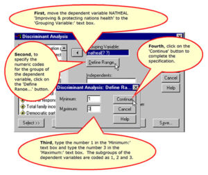
Each dependent variable is a nonmetric variable that has three categories: 1 for “Spending too little”, 2 for “Spending about right”, and 3 for “Spending too much”.
In this exercise, we will use NATHEAL, “Improving & protecting nations health” , as the dependent variable.
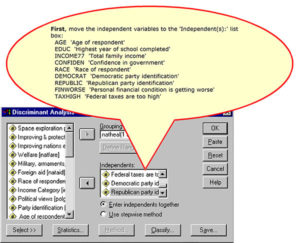
The independent variables are age, education, race, income, Democratic party identification, Republican party identification, confidence in government, personal financial situation worsening, and belief that federal taxes are too high.
The independent variables: race, democrat, republican, worsening financial situation, and taxes too high are nonmetric and have been already been converted to dummy-coded variables where necessary.
The independent variables: age, education, income, and confidence in government (a scaled variable) will be treated as metric variables.
Method for including independent variables
If we view the author’s intention as an interest in the role which these different factors play in attitude toward government spending, we want to see the results for all of the independent variables, so we use direct entry of all variables as our method of selection.
Stage 2: Develop the Analysis Plan: Sample Size Issues
In this stage, the following issues are addressed:
Missing data analysis
In the missing data analysis, we are looking for a pattern or process whereby the pattern of missing data could influence the results of the statistical analysis.
Run the MissingDataCheck Script
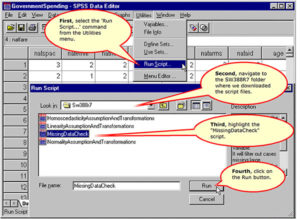
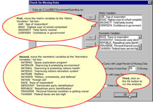
Complete the ‘Check for Missing Data’ Dialog Box
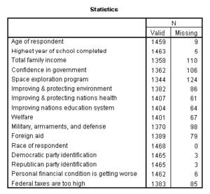
Number of Valid and Missing Cases per Variable
Three variables have over 100 missing cases: total family income, confidence in government, and spending on space exploration. However, because of the large sample size, all variables have valid data for 90% or more of cases, so no variables will be excluded for an excessive number of missing cases.
Frequency of Cases that are Missing Variables
Next, we examine the number of missing variables per case. Of the possible 16 variables in the missing data analysis (9 independent variables and 7 dependent variables), four cases were missing 8 or more variables, so we will exclude them from the analysis, reducing the sample size from 1468 to 1464.
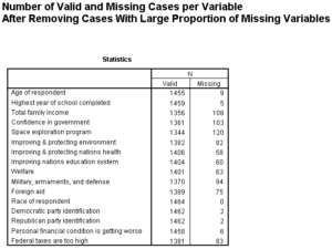
Number of Valid and Missing Cases after Removing Four Cases
After removing the four cases missing data for 50% or more of the variables, the number of valid cases for each variable is shown in the table below.
Distribution of Patterns of Missing Data
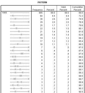
Correlation Matrix of Valid/Missing Dichotomous Variables
Inspection of the correlation matrix of valid/missing cases (not shown) reveals a single correlation close to the moderate range (0.394). This correlation is between two dependent variables, spending on military and spending on foreign aid, which will not be included in the same
analysis. All other correlations are in the weak or very weak range, so we can delete missing cases without fear that we are distorting the solution.
Minimum sample size requirement: 20+ cases per independent variable
The ratio of 1464 cases in the analysis to 9 independent variables is so large (163 to 1) that we will skip the more precise calculation taking into account the number of cases that will be missing in the analysis of each dependent variable.
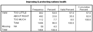
Division of the sample: 20+ cases in each dependent variable group
To compute the number of cases in each dependent variable group, we run a frequency distribution for that dependent variable. In the output, we see that the minimum group size is 112 cases, so we meet this requirement.
Stage 2: Develop the Analysis Plan: Measurement Issues:
In this stage, the following issues are addressed:
Incorporating Nonmetric Data with Dummy Variables
Dummy coding for all nonmetric variables was completed when the data set was created.
Representing Curvilinear Effects with Polynomials
We do not have any evidence of curvilinear effects at this point in the analysis.
Representing Interaction or Moderator Effects
We do not have any evidence at this point in the analysis that we should add interaction or moderator variables.
Stage 3: Evaluate Underlying Assumptions
In this stage, the following issues are addressed:
Nonmetric dependent variable and metric or dummy-coded independent variables
The dependent variable is nonmetric. All of the independent variables are metric or dichotomous dummy-coded variables.
Multivariate normality of metric independent variables
Since there is not a method for assessing multivariate normality, we assess the normality of the individual metric variables.
Run the ‘NormalityAssumptionAndTransformations’ Script
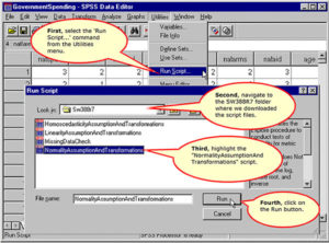
Complete the ‘Test for Assumption of Normality’ Dialog Box
Tests of Normality
We find that all of the independent variables fail the test of normality, and that none of the transformations induced normality in any variable. We should note the failure to meet the normality assumption for possible inclusion in our discussion of findings.
Linear relationships among variables
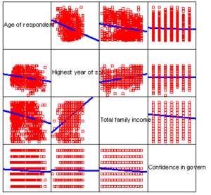
Since our dependent variable is not metric, we cannot use it to test for linearity of the independent variables. As an alternative, we can plot each metric independent variable against all other independent variables in a scatterplot matrix to look for patterns of nonlinear relationships. If one of the independent variables shows multiple nonlinear relationships to the other independent variables, we consider it a candidate for transformation
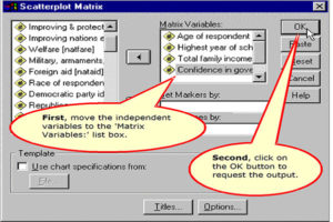
Requesting a Scatterplot Matrix
Specifications for the Scatterplot Matrix
The Scatterplot Matrix
Blue fit lines were added to the scatterplot matrix to improve interpretability.
None of the scatterplots show evidence of any nonlinear relationships.
Assumption of equal dispersion for dependent variable groups
Box’s M tests for homogeneity of dispersion matrices across the subgroups of the dependent variable. The null hypothesis is that the dispersion matrices are homogenous. If the analysis fails this test, we can request classification using separate group dispersion matrices in the classification phase of the discriminant analysis to see it this improves our accuracy rate.
Box’s M test is produced by the SPSS discriminant procedure, so we will defer this question until we have obtained the discriminant analysis output.
Stage 4: Estimation of Discriminant Functions and Overall Fit: The Discriminant Functions
In this stage, the following issues are addressed:
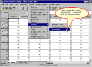
Compute the discriminant analysis
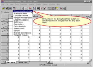
The steps to obtain a discriminant analysis are detailed on the following screens.
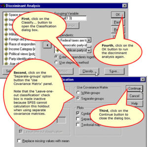
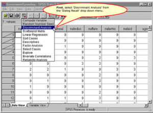
Requesting a Discriminant Analysis
Specifying the Dependent Variable
Specifying the Independent Variables
Specifying Statistics to Include in the Output
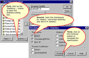
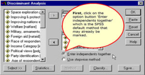
Specifying the Direct Entry Method for Selecting Variables
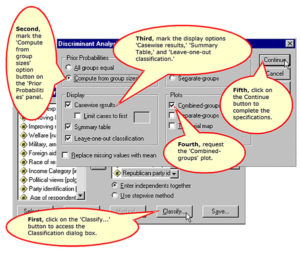
Specifying the Classification Options
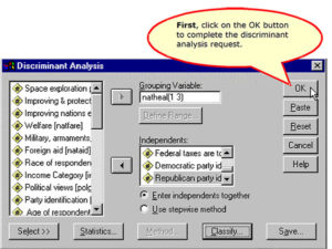
Complete the Discriminant Analysis Request
Overall significance of the discriminant function(s)
The output to determine the overall statistical significance of the discriminant functions is shown below. As we can see in the Wilks’ Lambda table, SPSS reports two statistically significant functions, with probabilities less than 0.05. Based on the Wilks’ Lambda tests, we would conclude that there is a statistically significant relationship between the independent and dependent variables, and there are two statistically significant discriminant functions.
The canonical correlation values of .276 for the first function and .130 for the second function match the values of .28 and .13 in the article.
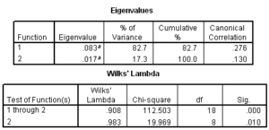
Our conclusion from this output is that there are two statistically significant discriminant functions for this problem.
Stage 4: Estimation of Discriminant Functions and Overall Fit: Assessing Model Fit
In this stage, the following issues are addressed:
Assumption of equal dispersion for dependent variable groups
In discriminant analysis, the best measure of overall fit is classification accuracy. The appropriateness of using the pooled covariance matrix in the classification phase is evaluated by the Box’s M statistic.
For this problem, Box’s M statistic is statistically significant, so we conclude that the dispersion of our two groups is not homogeneous.
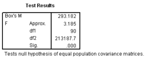
Since we failed this test, we will re-run the analysis using separate covariance matrices in classification and see if this improves our overall accuracy rate. We will compare the results of the modified analysis to the cross-validated accuracy rate of 57.2% obtained for this analysis, as shown in the following table.
Re-running the Discriminant Analysis using separate-groups covariance matrices
Requesting classification using separate-groups covariance matrices
Results of classification using separate-groups covariance matrices
The results of the classification using separate covariance matrices improves the accuracy of the model from 57.2% to 57.6%. This is equivalent to an improvement of 1% (.6/57.2). This is below the usual 10% improvement criteria that we require for a model with greater complexity and additional interpretive burden. We will revert to the model using pooled, or within-groups, covariance matrices for the classification phase of the analysis since we do not gain anything in the separate covariance model.
Classification accuracy by chance criteria
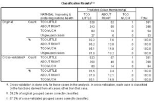
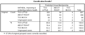
The Classification Results table is shown again for the model using pooled covariance matrices for classification.
As shown below, the classification accuracy for our analysis is 57.2% (using the cross-validated accuracy rate). The accuracy rate is not reported in the article.

Using hand calculations I computed the proportional by chance accuracy rate to be 0.459 (.581^2 + .339^2 + .080^2) using the proportion of cases reported in each group in the table of Prior Probabilities for Groups. A 25% increase over chance results in a benchmark of 0.574. I would interpret the cross-validated classification accuracy rate, 57.2%, as satisfying the proportional by chance accuracy criteria.
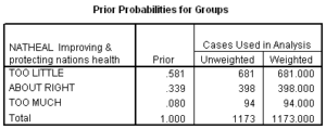
Since one of our groups, “Too Little,” makes up 58% of our sample in a three-group problem, it is appropriate to apply the maximum chance criteria, which I compute to be 0.726. We do not meet this criteria, so we should be cautious in generalizing the results of this model.
We should also note that much of the model’s accuracy was accomplished by predicting a large proportion of each group to be members of the dominant “Too Little” group. None of the “Too Much” cases were predicted accurately and only 12% of the “About Right” group was accurately predicted. Although we found two statistically significant discriminant functions separating the three groups, in fact, they were only achieving slight differentiation of the ‘Too little’ and ‘About right’ groups.
Press’s Q statistic
Substituting the parameters for this problem into the formula for Press’s Q, we obtain [1173-(675×3)] ^2 / (1173x(3-1)) = 309.4, which exceeds the critical value of 6.63. According to this statistic, our prediction accuracy is greater than expected by chance. However, as the text notes on page 205, this test is sensitive to sample size in much the same way that chi square values are affected by orders of magnitude (powers of ten, i.e. 10, 100, 1000, etc.). While this statistic is significant, the significance is a consequence of sample size as much as effect size. This is supported by the lack of relationship signified by the limited predictive accuracy.
Presence of outliers
SPSS print Mahalanobis distance scores for each case in the table of Casewise Statistics, so we can use this as a basis for detecting outliers.
We can request this figure from SPSS using the following compute command:
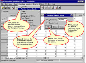
COMPUTE mahcutpt = IDF.CHISQ(0.99,9). EXECUTE.
Where 0.99 is the cumulative probability up to the significance level of interest and 9 is the number of degrees of freedom. SPSS will create a column of values in the data set that contains the desired value.
We scan the table of Casewise Statistics to identify any cases that have a Squared Mahalanobis distance greater than 21.666 for the group to which the case is most likely to belong, i.e. under the column labeled ‘Highest Group.’
Scanning the Casewise Statistics for the Original sample (not shown), I do not find any cases which have a D2 value this large for the highest classification group. The largest value I found was 16.165.
Stage 5: Interpret the Results
In this section, we address the following issues:
Number of functions to be interpreted
As indicated previously, there are two significant discriminant functions to be interpreted.
Role of functions in differentiating categories of the dependent variable
The combined-groups scatterplot enables us to link the discriminant functions to the categories of the dependent variable. I have modified the SPSS output by changing the symbols for the different points so that we can detect the group members on a black and white page. In addition, I have added reference lines at the zero value for each axis.
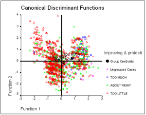
Analyzing this plot, we see that the first function differentiates the ‘Too Little’ group from ‘About Right’ and ‘Too Much’ groups. The second function differentiates the ‘Too Much’ group from the ‘About Right’ group.
Assessing the contribution of predictor variables
Identifying the statistically significant predictor variables
When we do direct entry of all the independent variables, we do not get a statistical test of the significance of the contribution of each individual variable. While we could run the stepwise procedure to obtain these tests, we can also look to the structure matrix for an indication of the importance of variables.
Importance of Variables and the Structure Matrix
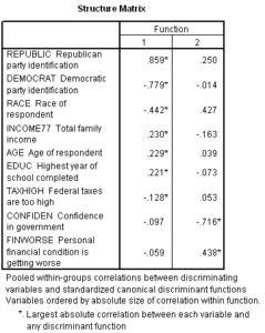
The Structure Matrix is a matrix of the correlations between the individual predictors and the discriminant functions. These correlations are also referred to as the discriminant loadings and can be interpreted like factor loadings in assessing the relative contribution of each independent variable to the discriminant function. While there is not a consensus on the size of loading required for interpretation, Tabachnick and Fidell state “By convention, correlations in excess of 0.33 (10% of variance) may be considered eligible while lower ones are not.” (page 540).
Following this guideline, we would identify three variables as important to the first discriminant function: REPUBLIC ‘Republican party identification’, DEMOCRAT ‘Democratic party identification’, and RACE ‘Race of respondent’.
We would identify CONFIDEN ‘Confidence in government’ and FINWORSE ‘Personal financial Conditions is getting worse’ as important to the second discriminant function
Note that our purpose in examining the structure matrix in discriminant analysis is not the same as our purpose in factor analysis, so we do not have the concern with simple structure in identifying important predictor variables that we had with factor analysis. A variable can play multiple roles in the discriminant functions, e.g. higher than average scores can be associated with membership is one group, while lower than average scores can be associated with membership in another group.
Comparing Group Means to Determine Direction of Relationships
We can examine the pattern of means on the significant independent for the three groups of the dependent variable to identify the role of the independent variables in predicting group membership. The following table contains an extract of the SPSS output of the group statistics.
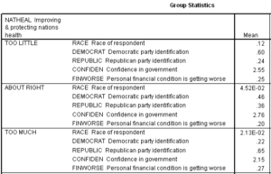
The first discriminant function distinguishes the groups ‘Too Little’ from ‘About Right’ and ‘Too Much’. Persons choosing the ‘Too Little’ response were more likely to be Black (12% versus 5% of the About Right group and 2% of the ‘Too Much’ group). Similarly, they were more likely to identify with the Democratic party (60% versus 46% and 22%) and less likely to identify with the Republican party (24% versus 36% and 65%).
The second discriminant function distinguishes the groups ‘About Right’ from ‘Too Little’ and ‘Too Much.’ The ‘About Right’ group had a higher average score on confidence in government (2.76 to 2.55 and 2.15) and had a lower proportion of respondents who thought that their personal financial situation was getting worse (20% versus 25% and 27%)
Impact of Multicollinearity on solution
Multicollinearity is indicated by SPSS for discriminant analysis by very small tolerance values for variables, e.g. less than 0.10 (0.10 is the size of the tolerance, not its significance value).
When we request direct entry of all independent variables, SPSS does not print out tolerance values as it does for stepwise entry. However, if a variable is collinear with another independent variable, SPSS will not enter it into the discriminant functions, but will instead print out a table in the output like the following:
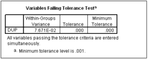
To force SPSS to print, this table I created a duplicate variable named DUP that had the same values as another independent variable.
Since we do not find a table like this in our output, we can conclude that multicollinearity is not a problem in this analysis.
Stage 6: Validate The Model
In this stage, we are normally concerned with the following issues:
Conducting the Validation Analysis
To validate the discriminant analysis, we can randomly divide our sample into two groups, a screening sample and a validation sample. The analysis is computed for the screening sample and used to predict membership on the dependent variable in the validation sample. If the model is valid, we would expect that the accuracy rates for both groups would be about the same.
In the double cross-validation strategy, we reverse the designation of the screening and validation sample and re-run the analysis. We can then compare the discriminant functions derived for both samples. If the two sets of functions contain a very different set of variables, it indicates that the variables might have achieved significance because of the sample size and not because of the strength of the relationship. Our findings about these individual variables would that the predictive utility of these predictors is not generalizable.
Set the Starting Point for Random Number Generation
Compute the Variable to Randomly Split the Sample into Two Halves
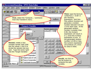
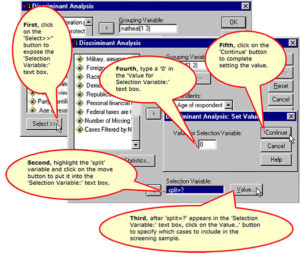
Specify the Cases to Include in the First Screening Sample
Specify the Value of the Selection Variable for the First Validation Analysis
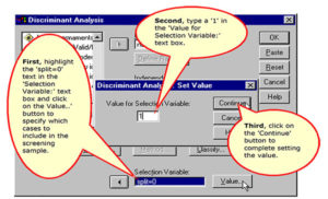
Specify the Value of the Selection Variable for the Second Validation Analysis
Generalizability of the Discriminant Model
We base our decisions about the generalizability of the discriminant model on a table which compares key outputs comparing the analysis with the full data set to each of the validation runs.
|
|
Full Model |
Split=0 |
Split=1 |
|
Number of Significant Functions |
2 |
1 |
1 |
|
Cross-validated Accuracy for |
57.2% |
57.0% |
57.8% |
|
Accuracy Rate for |
|
58.2% |
56.5% |
|
Important Variables from |
REPUBLIC DEMOCRAT RACE CONFIDEN FINWORSE
|
SPSS output is for two functions, |
SPSS output is for two functions, |
The accuracy rate of the model is maintained throughout the validation analysis, suggesting that this is a correct assessment of our ability to predict attitude toward health spending.
However, a second discriminant function was not found in either of the validation analyses, suggesting that the significance of the second function in the model of the full data set was associated with the larger sample size in that analysis.
The failure to validate the second function implies that the data only supports the existence of the first discriminant function which differentiates the group that feels we are spending ‘Too Little’ on health care from other respondents. In addition the accuracy of the model is based on it classification of all cases in the ‘Too Little’ group. The accuracy rate of the discriminant model could be achieved by chance alone.
In sum, our ability to differentiate preferences for health spending is limited by the fact that most respondents to the survey believe we should spend more on health care. The independent variables available in this analysis are not good discriminators of different preferences for health spending.