
This is the sample problem presented in the text on pages 314 to 321. Consistent with the authors’ strategy for presenting the problem, we will divide the data set into a learning sample and a validation sample, after a brief overview of logistic regression.
overview of logistic regression.
Multiple regression requires that the dependent variable be a metric variable. There are, however, many problems in which the dependent variable is a non-metric class or category and the goal of our analysis is to produce a model that predicts group membership or classification. For example, we might be interested in predicting whether individuals will succeed or fail in some treatment, i.e. the likelihood that they will be a member of a particular outcome group.
We will look at two strategies for addressing this type of problem: discriminant analysis and logistic regression. Discriminant analysis can be used for any number of groups. Logistic regression is commonly used with two groups, i.e. the dependent variable is dichotomous. Discriminant analysis requires that our data meet the assumptions of multivariate normality and equality of variance-covariance across groups. Logistic regression does not require these assumptions: “In logistic regression, the predictors do not have to be normally distributed, linearly related, or of equal variance within each group.” (Tabachnick and Fidell, page 575)
Logistic regression predicts the probability that the dependent variable event will occur given a subject’s scores on the independent variables. The predicted values of the dependent variable can range from 0 to 1. If the probability for an individual case is equal to or above some threshold, typically 0.50, then our prediction is that the event will occur. Similarly, if the probability for an individual case is less than 0.50, then our prediction is that the event will not occur. One of the criticisms of logistic regression is that its group prediction does not take into account the relative position of a case within the distribution, a case that has a probability of .51 is classified in the same group as a case that has a probability of .99, since both are above the .50 cutoff.
The dependent variable plotted against the independent variables follows an s-shaped curve, like that shown in the text on page 277. The relationship between the dependent and independent variable is not linear.
As with multiple regression, we are concerned about the overall fit, or strength of the relationship between the dependent variable and the independent variables, but the statistical measures of the fit are different than those employed in multiple regression. Instead of the F-test for overall significance of the relationship, we will interpret the Model Chi-Square statistic which is the test of a model which has no independent variables versus a model that has independent variables. There is a “pseudo R square” statistic that can be computed and interpreted as an R square value. We can also examine a classification table of predicted versus actual group membership and use the accuracy of this table in evaluating the utility of the statistical model.
The coefficients for the predictor variables measure the change in the probability of the occurrence of the dependent variable event in log units. Since the B coefficients are in log units, we cannot directly interpret their meaning as a measure of change in the dependent variable. However, when the B coefficient is used as a power to which the natural log (2.71828) is raised, the result represents an odds ratio, or the probability that an event will occur divided by the probability that the event will not occur. If a coefficient is positive, its transformed log value will be greater than one, meaning that the event is more likely to occur. If a coefficient is negative, its transformed log value will be less than one, and the odds of the event occurring decrease. A coefficient of zero (0) has a transformed log value of 1.0, meaning that this coefficient does not change the odds of the event one way or the other. We can state the information in the odds ratio for dichotomous independent variables as: subjects having or being the independent variable are more likely to have or be the dependent variable, assuming the that a code of 1 represents the presence both the independent and the dependent variable. For metric independent variables, we can state that subjects having more of the independent variable are more likely to have or be the dependent variable, assuming that the independent variable and the dependent variable are both coded in this direction.
There are several numerical problems that can occur in logistic regression that are not detected by SPSS or other statistical packages: multicollinearity among the independent variables, zero cells for a dummy-coded independent variable because all of the subjects have the same value for the variable, and “complete separation” whereby the two groups in the dependent event variable can be perfectly separated by scores on one or a combination of the independent variables. All of these problems produce large standard errors (I recall the threshold as being over 2.0, but I am unable to find a reference for this number) for the variables included in the analysis and very often produce very large B coefficients as well. If we encounter large standard errors for the predictor variables, we should examine frequency tables, one-way ANOVAs, and correlations for the variables involved to try to identify the source of the problem.
Like multiple regression and discriminant analysis, we are concerned with detecting outliers and influential cases and the effect that they may be having on the model. Finally, we can use diagnostic plots to evaluate the fit of the model to the data and to identify strategies for improving the relationship expressed in the model.
Sample size, power, and the ratio of cases to variables are important issues in logistic regression, though the specific information is less readily available. In the absence of any additional information, we may employ the standards required for multiple regression.
Preliminary Division of the Data Set
The data for this problem is the Hatco.Sav data set.
Instead of conducting the analysis with the entire data set, and then splitting the data for the validation analysis, the authors opt to divide the sample prior to doing the analysis. They use the estimation or learning sample of 60 cases to build the discriminant model and the other 40 cases for a holdout sample to validate the model.
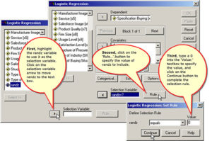
To replicate the author’s analysis, we will create a randomly generated variable, randz, to split the sample. We will use the cases where randz = 0 to create the logistic regression model and apply that model to the validation sample to estimate the model’s true accuracy rate.
Note the results produced in the chapter example were obtained by using the same random seed and compute statement as the two-group discriminant analysis, not the SPSS syntax commands specified in the text on page 707.
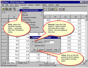
Specify the Random Number Seed
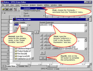
Compute the random selection variable
Stage One: Define the Research Problem
In this stage, the following issues are addressed:
- Relationship to be analyzed
- Specifying the dependent and independent variables
- Method for including independent variables
Relationship to be analyzed
The research problem is still to determine if differences in perception of HATCO can distinguish between customers using specification buying versus total value analysis (text, page 314).
Specifying the dependent and independent variables
The dependent variable is
- X11 ‘Purchasing Approach’,
a dichotomous variable, where 1 indicates “Total Value Analysis” and 0 indicates “Specification Buying.”
The independent variables are:
- X1 ‘Delivery Speed’
- X2 ‘Price Level’
- X3 ‘Price Flexibility’
- X4 ‘Manufacturer Image’
- X5 ‘Service’
- X6 ‘Salesforce Image’
- X7 ‘Product Quality
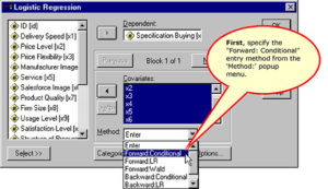
Method for including independent variables
Since the authors are interested in the best subset of predictors, they use the forward stepwise method for selecting independent variables.
Stage 2: Develop the Analysis Plan: Sample Size Issues
In this stage, the following issues are addressed:
- Missing data analysis
- Minimum sample size requirement: 15-20 cases per independent variable
Missing data analysis
There is no missing data in this problem.
Minimum sample size requirement: 15-20 cases per independent variable
The data set has 60 cases and 7 independent variables for a ratio of 9 to 1, short of the requirement that we have 15-20 cases per independent variable.
Stage 2: Develop the Analysis Plan: Measurement Issues:
In this stage, the following issues are addressed:
- Incorporating nonmetric data with dummy variables
- Representing Curvilinear Effects with Polynomials
- Representing Interaction or Moderator Effects
Incorporating Nonmetric Data with Dummy Variables
All of the independent variables are metric.
Representing Curvilinear Effects with Polynomials
We do not have any evidence of curvilinear effects at this point in the analysis.
Representing Interaction or Moderator Effects
We do not have any evidence at this point in the analysis that we should add interaction or moderator variables.
Stage 3: Evaluate Underlying Assumptions
In this stage, the following issues are addressed:
- Nonmetric dependent variable with two groups
- Metric or dummy-coded independent variables
Nonmetric dependent variable having two groups
The dependent variable is X11 ‘Purchasing Approach’, a dichotomous variable, where 1 indicates “Total Value Analysis” and 0 indicates “Specification Buying.”
Metric or dummy-coded independent variables
All of the independent variables in the analysis are metric: X1 ‘Delivery Speed’, X2 ‘Price Level’, X3 ‘Price Flexibility’, X4 ‘Manufacturer Image’, X5 ‘Service’, X6 ‘Salesforce Image’, and X7 ‘Product Quality
Stage 4: Estimation of Logistic Regression and Assessing Overall Fit: Model Estimation
In this stage, the following issues are addressed:
- Compute logistic regression model
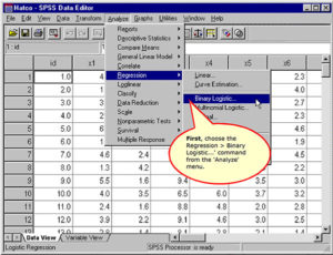
Compute the logistic regression
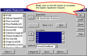
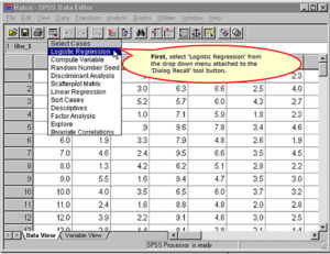
The steps to obtain a logistic regression analysis are detailed on the following screens.
Requesting a Logistic Regression
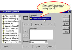
Specifying the Dependent Variable
Specifying the Independent Variables

Specify the method for entering variables
Specifying Options to Include in the Output
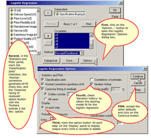
Specifying the New Variables to Save
Specifying the cases to include in the analysis
Complete the Logistic Regression Request
Stage 4: Estimation of Logistic Regression and Assessing Overall Fit: Assessing Model Fit
In this stage, the following issues are addressed for the stepwise inclusion of variables:
- Significance test of the model log likelihood (Change in -2LL)
- Measures Analogous to R2: Cox and Snell R2 and Nagelkerke R2
- Classification matrices
- Check for Numerical Problems
Once we have decided on the number of variables to be included in the equation, we will examine other issues of fit and compare model accuracy to the by chance accuracy rates.
- Hosmer-Lemeshow Goodness-of-fit
- By chance accuracy rates
- Presence of outliers
Step 1 of the Stepwise Logistic Regression Model
In this section, we will examine the results obtained at the first step of the analysis.
Initial statistics before independent variables are included
The Initial Log Likelihood Function, (-2 Log Likelihood or -2LL) is a statistical measure like total sums of squares in regression. If our independent variables have a relationship to the dependent variable, we will improve our ability to predict the dependent variable accurately, and the log likelihood value will decrease. The initial –2LL value is 78.859 on step 0, before any variables have been added to the model.
Significance test of the model log likelihood
At step 1, the variable X7 ‘Product Quality’ is added to the logistic regression equation. The addition of this variable reduces the initial log likelihood value (-2 Log Likelihood) of 78.859 to 37.524.
The difference between these two measures is the model child-square value (41.335 = 78.859 – 37.524) that is tested for statistical significance. This test is analogous to the F-test for R2 or change in R2 value in multiple regression which tests whether or not the improvement in the model associated with the additional variables is statistically significant.
In this problem the Model Chi-Square value of 41.335 has a significance of less than 0.0001, less than 0.05, so we conclude that there is a significant relationship between the dependent variable and the set of independent variables, which includes a single variable at this step.
Measures Analogous to R2
The next SPSS outputs indicate the strength of the relationship between the dependent variable and the independent variables, analogous to the R2 measures in multiple regression.
The Cox and Snell R2 measure operates like R2, with higher values indicating greater model fit. However, this measure is limited in that it cannot reach the maximum value of 1, so Nagelkerke proposed a modification that does range from 0 to 1. We will rely upon Nagelkerke’s measure as indicating the strength of the relationship.
If we applied our interpretive criteria to the Nagelkerke R2 of 0.681, we would characterize the relationship as very strong.
The Classification Matrices
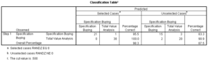
The classification matrices in logistic regression serve the same function as the classification matrices in discriminant analysis, i.e. evaluating the accuracy of the model.
If the predicted and actual group memberships are the same, i.e. 1 and 1 or 0 and 0, then the prediction is accurate for that case. If predicted group membership and actual group membership are different, the model “misses” for that case. The overall percentage of accurate predictions (85.00% in this case) is the measure of the model that we rely on most heavily fin logistic regression because it has a meaning that is readily communicated, i.e. the percentage of cases for which our model predicts accurately.
Correspondence of Actual and Predicted Values of the Dependent Variable
The final measure of model fit is the Hosmer and Lemeshow goodness-of-fit statistic, which measures the correspondence between the actual and predicted values of the dependent variable. In this case, better model fit is indicated by a smaller difference in the observed and predicted classification. A good model fit is indicated by a nonsignificant chi-square value.
At step 1, the Hosmer and Lemshow Test is not statistically significant, indicating predicted group memberships correspond closely to the actual group memberships, indicating good model fit.
Check for Numerical Problems
There are several numerical problems that can occur in logistic regression that are not detected by SPSS or other statistical packages: multicollinearity among the independent variables, zero cells for a dummy-coded independent variable because all of the subjects have the same value for the variable, and “complete separation” whereby the two groups in the dependent event variable can be perfectly separated by scores on one or a combination of the independent variables.
All of these problems produce large standard errors (over 2) for the variables included in the analysis and very often produce very large B coefficients as well. If we encounter large standard errors for the predictor variables, we should examine frequency tables, one-way ANOVAs, and correlations for the variables involved to try to identify the source of the problem.
Our final step, in assessing the fit of the derived model is to check the coefficients and standard errors of the variables included in the model.
For the single variable included on the first step, neither the standard error nor the B coefficient are large enough to suggest any problem.
Step 2 of the Stepwise Logistic Regression Model
Significance test of the model log likelihood
At step 2, the variable X3 ‘Price Flexibility’ is added to the logistic regression equation. The addition of this variable reduces the initial log likelihood value (-2 Log Likelihood) of 78.858931 to 20.258.
The difference between these two measures is the model child-square value (58.601 = 78.859 – 20.258) that is tested for statistical significance. This test is analogous to the F-test for R2 or change in R2 value in multiple regression which tests whether or not the improvement in the model associated with the additional variables is statistically significant.
In this problem the Model Chi-Square value of 58.601 has a significance of less than 0.0001, less than 0.05, so we conclude that there is a significant relationship between the dependent variable and the set of independent variables, which now includes two independent variables at this step.
Measures Analogous to R2
The next SPSS outputs indicate the strength of the relationship between the dependent variable and the independent variables, analogous to the R2 measures in multiple regression.
If we applied our interpretive criteria to the Nagelkerke R2 of 0.852 (up from 0.681 at the first step), we would characterize the relationship as very strong.
The Classification Matrices
The classification matrices in logistic regression serve the same function as the classification matrices in discriminant analysis, i.e. evaluating the accuracy of the model.
The overall percentage of accurate predictions now increases to 98.33% in this case. Only one case is classified incorrectly.
Correspondence of Actual and Predicted Values of the Dependent Variable
The final measure of model fit is the Hosmer and Lemeshow goodness-of-fit statistic, which measures the correspondence between the actual and predicted values of the dependent variable. In this case, better model fit is indicated by a smaller difference in the observed and predicted classification. A good model fit is indicated by a nonsignificant chi-square value.
At step 2, the Hosmer and Lemshow Test is not statistically significant, indicating predicted group memberships correspond closely to the actual group memberships, indicating good model fit.
Check for Numerical Problems
Our check for numerical problems is a check for standard errors larger than 2 or unusually large B coefficients.
We do not identify any problems from the table of variables in the equation.
Step 3 of the Stepwise Logistic Regression Model
In this section, we will examine the results obtained at the third step of the analysis.
Significance test of the model log likelihood
At step 3, the variable X5 ‘Service’ is added to the logistic regression equation. The addition of this variable reduces the initial log likelihood value (-2 Log Likelihood) of 78.859 to 6.254.
The difference between these two measures is the model child-square value (72.605 = 78.859 – 6.254) that is tested for statistical significance. This test is analogous to the F-test for R2 or change in R2 value in multiple regression which tests whether or not the improvement in the model associated with the additional variables is statistically significant.
In this problem the Model Chi-Square value of 72.605 has a significance of less than 0.0001, less than 0.05, so we conclude that there is a significant relationship between the dependent variable and the set of independent variables, which now includes three independent variables at this step.
Measures Analogous to R2
The next SPSS outputs indicate the strength of the relationship between the dependent variable and the independent variables, analogous to the R2 measures in multiple regression.
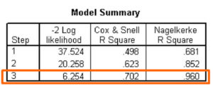
If we applied our interpretive criteria to the Nagelkerke R2 of 0.960 (up from 0.852 at the previous step), we would characterize the relationship as very strong.
Correspondence of Actual and Predicted Values of the Dependent Variable
The final measure of model fit is the Hosmer and Lemeshow goodness-of-fit statistic, which measures the correspondence between the actual and predicted values of the dependent variable. In this case, better model fit is indicated by a smaller difference in the observed and predicted classification. A good model fit is indicated by a nonsignificant chi-square value.

At step 3, the Hosmer and Lemshow Test is not statistically significant, indicating predicted group memberships correspond closely to the actual group memberships, indicating good model fit.
The Classification Matrices
The classification matrices in logistic regression serve the same function as the classification matrices in discriminant analysis, i.e. evaluating the accuracy of the model.
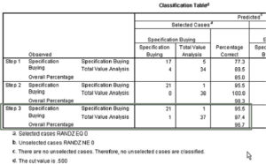
The overall percentage of accurate predictions for the three variable model is 98.33%. Only two cases are classified incorrectly.
Check for Numerical Problems
Our check for numerical problems is a check for standard errors larger than 2 or unusually large B coefficients.
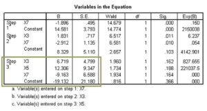
The standard errors for all of the variables in the model are substantially larger than 2, indicating a serious numerical problem. In addition, the B coefficients have become very large (remember that these are log values, so the corresponding decimal value would appear much larger).
This model should not be used, and we should interpret the model obtained at the previous step.
In hindsight, we may have gotten a notion that a problem would occur in this step from the classification table at the previous step. Recall that we had only one misclassification on the previous step, so there was almost no overlap remaining between the groups of the dependent variable.
Returning to the two-variable model
The residual and Cook’s distance measures which we have available are for the three variable model which SPSS was working with at the time it concluded the stepwise selection of variables. Since I do not know of a way to force SPSS to stop at step 2, I will repeat the analysis using direct entry for the two independent variables which were found to be significant with stepwise selection: X7 ‘Product Quality’ and X3 ‘Price Flexibility.’
Re-run the Logistic Regression
Complete the specification for the new analysis
The Two-Variable Model
To sum up evidence of model fit presented previously, the Model Chi-Square value of 58.601 has a significance of less than 0.0001, less than 0.05, so we conclude that there is a significant relationship between the dependent variable and the two independent variables. The Nagelkerke R2 of 0.852 would indicate that the relationship is very strong. The Hosmer and Lemeshow goodness-of-fit measure has a value of 10.334 which has the desirable outcome of nonsignificance.
The Classification Matrices
The classification matrices in logistic regression serve the same function as the classification matrices in discriminant analysis, i.e. evaluating the accuracy of the model.
The overall percentage of accurate predictions (98.33% in this case) is very high, with only one case being misclassified.
To evaluate the accuracy of the model, we compute the proportional by chance accuracy rate and the maximum by chance accuracy rates, if appropriate.
The proportional by chance accuracy rate is equal to 0.536 (0.633^2 + 0.367^2). A 25% increase over the proportional by chance accuracy rate would equal 0.669. Our model accuracy race of 98.3% exceeds this criterion.
Since one of our groups contains 63.3% of the cases, we might also apply the maximum by chance criterion. A 25% increase over the largest groups would equal 0.792. Our model accuracy race of 98.3% also exceeds this criterion.
In addition, the accuracy rates for the unselected validation sample, 87.50%, surpasses both the proportional by chance accuracy rate and the maximum by chance accuracy rate.
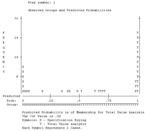
SPSS provides a visual image of the classification accuracy in the stacked histogram as shown below. To the extent to which the cases in one group cluster on the left and the other group clusters on the right, the predictive accuracy of the model will be higher.
Presence of outliers
There are two outputs to alert us to outliers that we might consider excluding from the analysis: listing of residuals and saving Cook’s distance scores to the data set.
SPSS provides a casewise list of residuals that identify cases whose residual is above or below a certain number of standard deviation units. Like multiple regression there are a variety of ways to compute the residual. In logistic regression, the residual is the difference between the observed probability of the dependent variable event and the predicted probability based on the model. The standardized residual is the residual divided by an estimate of its standard deviation. The deviance is calculated by taking the square root of -2 x the log of the predicted probability for the observed group and attaching a negative sign if the event did not occur for that case. Large values for deviance indicate that the model does not fit the case well. The studentized residual for a case is the change in the model deviance if the case is excluded. Discrepancies between the deviance and the studentized residual may identify unusual cases. (See the SPSS chapter on Logistic Regression Analysis for additional details).
In the output for our problem, SPSS listed one case that may be considered an outlier with a studentized residuals greater than 2, case 13:
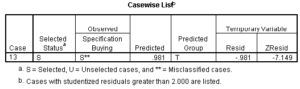
SPSS has an option to compute Cook’s distance as a measure of influential cases and add the score to the data editor. I am not aware of a precise formula for determining what cutoff value should be used, so we will rely on the more traditional method for interpreting Cook’s distance which is to identify cases that either have a score of 1.0 or higher, or cases which have a Cook’s distance substantially different from the other. The traditional method for detecting unusually large Cook’s distance scores is to create a scatterplot of Cook’s distance scores versus case id or case number.
Request the Scatterplot of Cook’s Distances
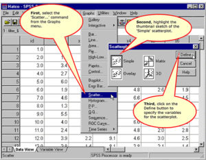
Specifying the Variables for the Scatterplot
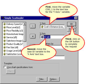
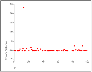
The Scatterplot of Cook’s Distances
On the plot of Cook’s distances, we see a case that exceeds the 1.0 rule of thumb for influential cases and has a distance value much different than the other cases. This is actually the same case that was identified as an outlier on the casewise plot, though it is difficult to track down because SPSS uses the case number in the learning sample for the casewise plot.
This case is the only case in the two variable model that was misclassified. We cannot omit it because we would again be faced with no overlap between the groups, producing the problematic numeric results that we found with the three variable model.
Stage 5: Interpret the Results
In this section, we address the following issues:
- Identifying the statistically significant predictor variables
- Direction of relationship and contribution to dependent variable
Identifying the statistically significant predictor variables
The coefficients are found in the column labeled B, and the test that the coefficient is not zero, i.e. changes the odds of the dependent variable event is tested with the Wald statistic, instead of the t-test as was done for the individual B coefficients in the multiple regression equation.

The Wald tests for the two independent variables X7 ‘Product Quality’ and X3 ‘Price Flexibility’ are both statistically significant (p < 0.05), as we knew they would be from the first two steps of the stepwise procedure.
Direction of relationship and contribution to dependent variable
The negative sign of X7 ‘Product Quality’ indicates an inverse relationship with the dependent variable. As the rating for X7 ‘Product Quality’ increases, there is a higher likelihood that the respondent favored the ‘Specification Buying’ approach to purchasing. In contrast the positive coefficient for X3 ‘Price Flexibility’ indicates a direct relationship to the dependent variable. As the rating for X3 ‘Price Flexibility’, there is a higher likelihood that the respondent favored the ‘Total Value Analysis’ approach to purchasing.
Since the B coefficient is expressed in log units, we cannot directly interpret the magnitude of the change associated with a one unit change in the independent variable. However, if we convert the B coefficient from log to decimal units, the result represents the change in the odds of having the dependent variable event for a one unit of change in the independent variable. For a one-unit change in X3 ‘Price Flexibility’, the odds of being in the ‘Total Value Analysis’ approach to purchasing increase by 6 times. A one unit change in X7 ‘Product Quality’ reduces the odds of being in the ‘Total Value Analysis’ approach to purchasing by 1/20th (i.e. you have a much lower probability of being in the ‘Total Value Analysis’ approach to purchasing).
Should we want to talk about the odds ratio for a different level of change, e.g. a 2-unit change in the independent variable, we cannot simply multiply the odds-ratio for a one unit change by 2. Instead we would multiply the B coefficient by 2 and take the antilog EXP(B) of that value. For example, in this problem, EXP(1×1.8035) = 6.2371, while the odds ratio for a two unit change in X3 would be EXP(2×1.8035) = 38.900.
Stage 6: Validate The Model
By holding out 40% of the subjects as a validation sample, the authors created the context for validation analysis. As stated above, the accuracy rate for the validation sample (87.50%) is in the same range as the accuracy rate for the learning sample (98.33%). Though the difference is larger than 10%, the very high accuracy rates for both samples would incline us to support a conclusion that the findings are generalizable.