
The purpose of this introductory example from pages 149-158 of the text is to demonstrate the basic concepts of regression analysis as one attempts to develop a predictive equation containing several independent variables. The dependent variable is the number of credit cards held by a family. The independent variables are family size and family income.
Prediction without an Independent Variable
With no information other than the number of credit cards per family, i.e. we only know the values for the dependent variable, Number of Credit Cards, our best estimate of the number of cards in a family is the mean. The cumulative amount of error in our guesses for all subjects in the data set is the sum of squared errors (squares of deviations from the mean).
Recall that variance equals the sum of squared errors divided by (the number of cases minus 1 degree of freedom). While we cannot obtain the sum of squared errors directly, we can compute the variance and multiply it by the number of cases in our sample minus 1.
Computing the Mean and Variance with SPSS
Request the Mean and Variance
The Descriptives Output
In the SPSS Output Navigator, we see that the variance is 3.143. If we multiply the variance by 7 (the number of cases in the study, 8 – 1 = 7), we compute the sum of squared errors to be equal to 22, which agrees with the text on page 151. If we use the mean for our best guess for each case, our measure of error is 22 units. The goal of regression is to use information from independent variables to reduce the amount of error associated with our guesses for the value of the dependent variable.

Prediction with One Independent Variable
A regression with a single independent variable and a dependent variable is referred to as simple linear regression.
Requesting a Simple Linear Regression
Simple Linear Regression Output
The regression coefficients are shown in the section of output shown below in the column titled ‘B’ of the coefficients table.
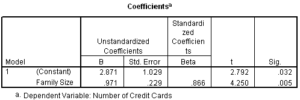
The coefficient for the independent variable Family Size is .971. The intercept is labeled as the (Constant) which is 2.871. If we were to write the regression equation, it would be:
Number of Credit Cards = 2.871 + 0.971 x Family Size
The ANOVA table provides the information on the sum of squared errors.
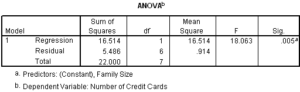
The ‘Total’ error or sum of squares (22) agrees with the calculation above for variance about the mean. When we use the information about the family size variable in estimating number of credit cards, we reduce the error in predicting number of credit cards to the ‘Residual’ sum of squares of 5.486 units. The difference between 22 and 5.486, 16.514, is the sum of squares attributed to the ‘Regression’ relationship between family size and number of credit cards.
The ratio of the sum of squares attributed to the regression relationship (16.514) to the total sum of squares (22.0) is equal to the value of R Square in the Model Summary Table, i.e. 16.514 / 22.0 = 0.751.
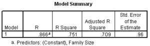
We would say that the pattern of variance in the independent variable, Family Size, explains 75.1% of the variance in the dependent variable, Number of Credit Cards.
Prediction with Two Independent Variables
Extending our analysis, we add another independent variable, Family Income, to the analysis. When we have more than one independent variable in the analysis, we refer to it as multiple regression.
Requesting a Multiple Regression
Requesting a Correlation Matrix
Multiple Regression Output
We will examine the correlation matrix before we review the regression output:
The ability of an independent variable to predict the dependent variable is based on the correlation between the independent and the dependent variable. When we add another independent variable, we must also concern ourselves with the intercorrelation between the independent variables.
If the independent variables are not correlated at all, their combined predictive power is the sum of their individual correlations. If the independent variables are perfectly correlated (co-linear), either one does an equally good job of predicting the dependent variable and the other is superfluous. When the intercorrelation is in between these extremes, the correlation among the independent variables can only be counted once in the regression relationship. When the second intercorrelated independent variable is added to the analysis, its relationship to the dependent variable will appear to be weaker than it really is because only the variance that it shares with the
dependent variable is incorporated into the analysis.
From the correlation matrix produced by the regression command above, we see that there is a strong correlation between ‘Family Size’ and ‘Family Income’ of 0.673. We expect ‘Family Income’ to improve our ability to predict ‘Number of Credit Cards’, but by a smaller amount than the 0.829 correlation between ‘Number of Credit Cards’ and ‘Family Income’ would suggest.
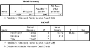
The remaining output from the regression command is shown below. The R Square measure of the strength of the relationship between the dependent variable and the independent variables increased by 0.110 (0.861 – 0.751 for the single variable regression).
The significance of the F statistic produced by the Analysis of Variance test (.007) indicates that there is a relationship between the dependent variable and the set of independent variables. The Sum of Squares for the residual indicates that we reduced our measure of error from 5.486 for the one variable equation, to 3.050 for the two variable equation.
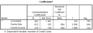
However, the significance tests of individual coefficients in the ‘Coefficients’ table tells us that the variable ‘Family Income’ does not have a statistically significant individual relationship with the dependent variable (Sig = 0.102). If we used an alpha level of 0.05, we would fail to reject the null hypothesis that the coefficient B is equal to 0.
When we
interpret multiple regression output, we must examine the significance test for the relationship between the dependent variable and the set of independent variables, the ANOVA test of the regression model, and the significance tests for individual variables in the Coefficients table. Understanding the patterns of relationships that exist among the variables requires that we consider the combined results of all significance tests.
Prediction with Three Independent Variables
Extending our analysis, we add another independent variable, Number of Automobiles Owned, to the analysis.
Requesting a Multiple Regression
Multiple Regression Output
The R Square for the two variable model was 0.861. Adding the third variable only increased the proportion of variance explained in the dependent variable by 1%, to 0.872.
The
significance of the F statistic produced by the Analysis of Variance test (.029) indicates that there is a relationship between the dependent variable and the set of three independent variables. The Sum of Squares for the residual indicates that we reduced our measure of error from 3.050 for the two variable equation, to 2.815 for the
three variable equation.
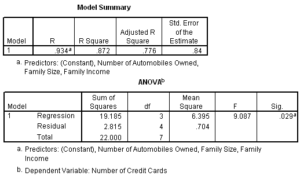
However, the significance tests of individual coefficients in the ‘Coefficients’ table tells us that both the second variable added ‘Family Income’ (Sig. = 0.170) and the third variable added ‘Number of Automobiles Owned’ (Sig. = 0.594) do not have a statistically significant individual relationship with the dependent variable
From this example, we see that the objective of multiple regression is to add independent variables to the regression equation that improve our ability to predict the dependent variable, by reducing the residual sum of squared errors between the predicted and actual values for the dependent variable. Ideally, all of the variables in our regression equation would have a significant individual relationship to the dependent variable.